Abstract -- Modeling robot motion planning with uncertainty in a Bayesian framework leads to a computationally intractable stochastic control problem. We seek hypotheses that can justify a separate implementation of control, localization and planning. In the end, we reduce the stochastic control problem to path-planning in the extended space of poses x covariances; the transitions between states are modeled through the use of the Fisher information matrix. In this framework, we consider two problems: minimizing the execution time, and minimizing the final covariance, with an upper bound on the execution time. Two correct and complete algorithms are presented. The first is the direct extension of classical graph-search algorithms in the extended space. The second one is a back-projection algorithm: uncertainty constraints are propagated backward from the goal towards the start state.

Additional material

• Master's thesis, May 2007 (PDF)

• C++ implementation of the method:

  • only the source code (600KB tgz)
  • the source code, plus the animations (15MB tgz)

Animations in Flash format

These are much fun to see! --- well, only if you are into planning.

The animations are Flash objects: use the left and right arrows to make the search process go back and forward. I did not make an MPEG video for ICRA with these, because it would take well over 5MB to present these with a good resolution. The animations are also available in PDF format -- click the link under the Flash object.

Environment shown in the paper

• Planning without uncertainty (for comparison):
  • A*
  • wavefront expansion
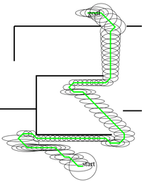
• Planning with uncertainty; solving PPU-MinTime:
  • forward search, A*
  • backward search, A*
  • backward search, wavefront expansion
• Planning with uncertainty; solving PPU-MinCov:
  • forward search, wavefront expansion

Another simple environment with non-orthogonal walls

• Planning without uncertainty (for comparison):
  • A*
  • wavefront expansion
• Planning with uncertainty; solving PPU-MinTime:
  • forward search, A*
  • backward search, A*
  • backward search, wavefront expansion
• Planning with uncertainty; solving PPU-MinCov:
  • forward search, wavefront expansion

Guided tour

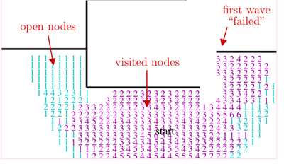
The animations show the number of nodes in the OPEN queue (turquoise numbers), and in the VISITED (closed) set (violet numbers).

For a start, you might want to take a look at PP without uncertainty using A*. Nothing surprising here, of course. But notice: for each pose, there is, at most, one node, in either the OPEN or VISITED set. This is because the dominance relation used is a total order. In this HTML text, let » be the dominance relation. Then, for simple PP, if n₁ and n₂ have the same pose, either n₁ » n₂ or n₂ » n₁.

This is not true when using A* to solve path planning with uncertainty (PPU). For example, in the same situation (env2-forward-A*), there are several nodes per cell in both OPEN and VISITED.

The point is that in PPU the covariance is part of the state space and should not be treated like another "cost". Once one gets this intuition, the rest is downhill.

There are many interesting sights to see, if you peruse through the animations. In env1-forward-A*, note the successive "waves" of nodes. The first waves that fail are the direct paths which are not localized enough.

Also in the case of env2-forward-A*, the search process tries to go straight to the goal, but no direct path is feasible. Then, a new path is tried, which differs slightly at the beginning, and then goes straight to the goal; this goes on until a path which acquires enough information is found.

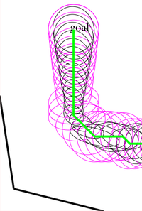
The backward algorithm is conceptually much more complicated. In this case, the nodes do not contain "states" (a pose + a covariance), but constraints on the states. However, graphically, they behave in the same way. See for example env2-backward-A*.

For the backward method, at the end of the animation there is a representation of the reverse path (q_k,{M_i}_k). The pink ellipses represent {M_i}_k -- the back-projection of CONSTRAINTS(q) -- and together they form an "envelope" in which the forward path (q_k, Σ_k) must pass.

It could happen (because of unmodelled phenomena), that, during execution, the actual covariance is different from the planned covariance. In that case, the planned path is still admissible and optimal, as long as the actual covariance is inside the envelope.